Welcome to the Optimizing Metrics section. This section goes over the different types of metrics that can be selected when training a new machine learning model as well as what values to look for in each metric type. When creating a new model the library will try to create the best performing model based on the selected metric.
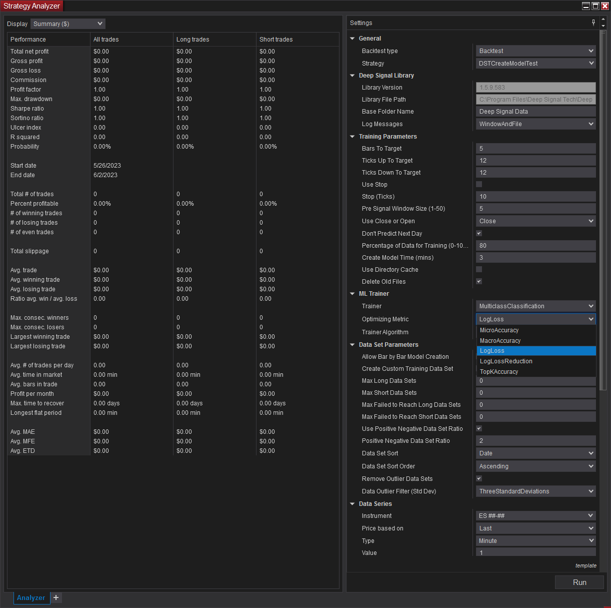
The Optimizing Metric can be selected under the ML Trainer section when creating a new model.
Here is a list of trainer types along with their associated optimizing metrics:
Binary Classification Metrics
Metrics |
Description |
Look For |
|
Accuracy |
Accuracy is the proportion of correct predictions with a test data set. It is the ratio of number of correct predictions to the total number of input samples. It works well if there are similar number of samples belonging to each class. |
The closer to 1.00, the better. But exactly 1.00 indicates an issue (commonly: label/target leakage, over-fitting, or testing with training data). When the test data is unbalanced (where most of the instances belong to one of the classes), the dataset is small, or scores approach 0.00 or 1.00, then accuracy doesn't really capture the effectiveness of a classifier and you need to check additional metrics. |
|
Area Under Roc Curve (AUC) |
AUC or Area under the curve measures the area under the curve created by sweeping the true positive rate vs. the false positive rate. |
The closer to 1.00, the better. It should be greater than 0.50 for a model to be acceptable. A model with AUC of 0.50 or less is worthless. |
|
Area Under Precision Recall Curve |
AUCPR or Area under the curve of a Precision-Recall curve: Useful measure of success of prediction when the classes are imbalanced (highly skewed datasets). |
The closer to 1.00, the better. High scores close to 1.00 show that the classifier is returning accurate results (high precision), and returning a majority of all positive results (high recall). |
|
F1 Score |
F1 score also known as balanced F-score or F-measure. It's the harmonic mean of the precision and recall. F1 Score is helpful when you want to seek a balance between Precision and Recall. |
The closer to 1.00, the better. An F1 score reaches its best value at 1.00 and worst score at 0.00. It tells you how precise your classifier is. |
|
Positive Precision |
Gets the positive precision of a classifier which is the proportion of correctly predicted positive instances among all the positive predictions (i.e., the number of positive instances predicted as positive, divided by the total number of instances predicted as positive). |
|
|
Positive Recall |
Gets the positive recall of a classifier which is the proportion of correctly predicted positive instances among all the positive instances (i.e., the number of positive instances predicted as positive, divided by the total number of positive instances). |
|
|
Negative Precision |
Gets the negative precision of a classifier which is the proportion of correctly predicted negative instances among all the negative predictions (i.e., the number of negative instances predicted as negative, divided by the total number of instances predicted as negative). |
|
|
Negative Recall |
Gets the negative recall of a classifier which is the proportion of correctly predicted negative instances among all the negative instances (i.e., the number of negative instances predicted as negative, divided by the total number of negative instances). |
|
For more details on binary classification, please see the following links:
Regression Metrics
Metrics |
Description |
Look For |
|
R-Squared |
R-squared (R2), or Coefficient of determination represents the predictive power of the model as a value between -inf and 1.00. 1.00 means there is a perfect fit, and the fit can be arbitrarily poor so the scores can be negative. A score of 0.00 means the model is guessing the expected value for the label. A negative R2 value indicates the fit does not follow the trend of the data and the model performs worse than random guessing. This is only possible with non-linear regression models or constrained linear regression. R2 measures how close the actual test data values are to the predicted values. |
The closer to 1.00, the better quality. However, sometimes low R-squared values (such as 0.50) can be entirely normal or good enough for your scenario and high R-squared values are not always good and be suspicious. |
|
Absolute-loss |
Absolute-loss or Mean absolute error (MAE) measures how close the predictions are to the actual outcomes. It is the average of all the model errors, where model error is the absolute distance between the predicted label value and the correct label value. This prediction error is calculated for each record of the test data set. Finally, the mean value is calculated for all recorded absolute errors. |
The closer to 0.00, the better quality. The mean absolute error uses the same scale as the data being measured (is not normalized to specific range). Absolute-loss, Squared-loss, and RMS-loss can only be used to make comparisons between models for the same dataset or dataset with a similar label value distribution. |
|
Squared-loss |
Squared-loss or Mean Squared Error (MSE), also called Mean Squared Deviation (MSD), tells you how close a regression line is to a set of test data values by taking the distances from the points to the regression line (these distances are the errors E) and squaring them. The squaring gives more weight to larger differences. |
It is always non-negative, and values closer to 0.00 are better. Depending on your data, it may be impossible to get a very small value for the mean squared error. |
|
RMS-loss |
RMS-Loss or Root Mean Squared Error (RMSE) (also called Root Mean Square Deviation, RMSD), measures the difference between values predicted by a model and the values observed from the environment that is being modeled. RMS-loss is the square root of Squared-loss and has the same units as the label, similar to the absolute-loss though giving more weight to larger differences. Root mean square error is commonly used in climatology, forecasting, and regression analysis to verify experimental results. |
It is always non-negative, and values closer to 0.00 are better. RMSD is a measure of accuracy, to compare forecasting errors of different models for a particular dataset and not between datasets, as it is scale-dependent. |
For more details on regression metrics, please see the following links:
Multiclass Classification Metrics
Metrics |
Description |
Look For |
|
Micro-Accuracy |
Micro-average Accuracy aggregates the contributions of all classes to compute the average metric. It is the fraction of instances predicted correctly. The micro-average does not take class membership into account. Basically, every sample-class pair contributes equally to the accuracy metric. |
The closer to 1.00, the better. In a multi-class classification task, micro-accuracy is preferable over macro-accuracy if you suspect there might be class imbalance (i.e you may have many more examples of one class than of other classes).. |
|
Macro-Accuracy |
Macro-average Accuracy is the average accuracy at the class level. The accuracy for each class is computed and the macro-accuracy is the average of these accuracies. Basically, every class contributes equally to the accuracy metric. Minority classes are given equal weight as the larger classes. The macro-average metric gives the same weight to each class, no matter how many instances from that class the dataset contains. |
The closer to 1.00, the better. It computes the metric independently for each class and then takes the average (hence treating all classes equally) |
|
Log-loss |
Logarithmic loss measures the performance of a classification model where the prediction input is a probability value between 0.00 and 1.00. Log-loss increases as the predicted probability diverges from the actual label. |
The closer to 0.00, the better. A perfect model would have a log-loss of 0.00. The goal of our machine learning models is to minimize this value. |
|
Log-Loss Reduction |
Logarithmic loss reduction can be interpreted as the advantage of the classifier over a random prediction. |
Ranges from -inf and 1.00, where 1.00 is perfect predictions and 0.00 indicates mean predictions. For example, if the value equals 0.20, it can be interpreted as "the probability of a correct prediction is 20% better than random guessing" |
For more details on Multi-class Classification metrics, please see the following links:
Source for metric information provided through Microsoft Machine Learning Resources
Futures, foreign currency and options trading contains substantial risk and is not for every investor. An investor could potentially lose all or more than the initial investment. Risk capital is money that can be lost without jeopardizing ones financial security or lifestyle. Only risk capital should be used for trading and only those with sufficient risk capital should consider trading. Past performance is not necessarily indicative of future results.